Dynamic and Static Light Scattering

Johannes Allwang

1 Light scattering (LS)

Static and dynamic light scattering (SLS and DLS) are powerful and widely employed optical characterization techniques that rely on the interaction of coherent light with density fluctuations in a small volume [1]. The origin of these density fluctuations can, for example, be polymers in solution, small particles in suspension, surfactant micelles, or subcellular biological components. Laser light scattering allows probing length-scales from nanometers to micrometers.

To allow instrument-independent interpretation of the data, the scattering vector \(\mathbf{q}\) and its absolute value, the momentum transfer \(q\) are defined as follows:

\[\begin{eqnarray} \mathbf{q} = \mathbf{k_f} - \mathbf{k_i}, && q = \left| \mathbf{q} \right| = \frac{4\pi n}{\lambda_l}\sin(\Theta) \tag{1.1} \end{eqnarray}\]

The raw signal in both SLS and DLS is the \(q\)-dependant intensity trace \(I(q, t)\). In SLS the time average \(\left<I(q, t)\right>_t\) is evaluated to get structural information about the scattering NPs while DLS uses the time-dependent auto-correlation of \(I(q, t)\) to extract information about their dynamics.

Fig. 1.1 shows a schematic representation of a light scattering setup. The incoming monochromatic laser beam (wavelength \(\lambda_l\)) has a wave-vector \(\mathbf{k_i}\) and hits the sample (in the present case the dispersion of NPs). The incoming laser light is scattered into all directions, but the figure shows only the relevant one. A detector is positioned at a scattering angle \(2\Theta\) and sample-to-detector distance \(sdd\). It detects the intensity \(I_f\) of the scattered laser beam, that has a wave vector \(\mathbf{k_f}\). Elastic scattering is assumed, so that \(\left|\mathbf{k_f}\right| = \left|\mathbf{k_i}\right|\).

Figure 1.1: Schematic representation of a light scattering setup. Incoming laser photons of wavelength \(\lambda_l\) are scattered into the detector. The scattered wave vector \(\mathbf{k_f}\) depends on the scattering angle \(2\Theta\).

1.1 Static light scattering (SLS)

In SLS the Rayleigh-ratio is calculated from the measured average intensites of the sample \(I_{\mathrm{sample}}(q) = \left<I_{\mathrm{sample}}(q, t)\right>_t\), the buffer \(I_{\mathrm{buffer}}(q) = \left<I_{\mathrm{buffer}}(q, t)\right>_t\) and a standard \(I_{\mathrm{std}}(q) = \left<I_{\mathrm{std}}(q, t)\right>_t\). In this , toluene is used as a standard.

The Rayleigh-ratio \(R(q)\) is defined as follows:

\[\begin{equation} R(q) = \left[I_{sample}(q) - I_{solvent}(q)\right]\frac{I_{std abs}}{I_{std}(q)} \tag{1.2} \end{equation}\]

\(I_{std abs}\) is a constant. The Rayleigh-ratio is directly proportional to the formfactor \(P(q)\) of the scattering particles:

\[\begin{equation} R(q) \propto P(q) \tag{1.3} \end{equation}\]

1.2 Dynamic light scattering (DLS)

DLS is based on Brownian motion and does not directly give structural information about the scattering particles. The fluctuations of the scattered intensity are used to find dynamic information about the sample, i.e. information about the Brownian motion of the scatterers. In case a diffusive process is observed, the Stokes-Einstein equation is used to relate the dynamic information to the size of the scatterers.

The setup used for DLS experiment (Fig. 1.2) is identical to the general LS-setup shown in Fig. 1.1, except that the detector has to collect the intensity as a function of time. Moreover, a correlator is used to calculate the auto-correlation function.

Figure 1.2: Schematic representation of a DLS setup. Incoming laser photons of wavelength \(\lambda_l\) are scattered into the detector. The scattered wave vector \(\mathbf{k_f}\) depends on the scattering angle \(2\Theta\). The signal is transformed into a correlation function by the correlator.

Figure 1.3 helps to illustrate the method: A bigger particle moves through the solution at a slower pace. The auto-correlation function goes to 0 for a higher delay time. We call the delay time, where the auto-correlation goes to 0 relaxation time \(\tau_D\). For a sample with big and small particles, there will be fast and slow fluctuations. The auto-correlation curve shows a double decay.

Figure 1.3: Illustrates typical intensity traces and corresponding auto-correlation functions for DLS measurements. The cyan and magenta curves correspond to bigger and smaller particles respectively. The green-yellow curve corresponds to the signal from big and small particles. code

Information about the diffusion coefficient can be extracted from the fluctuations of the measured intensity trace \(I(t, q)\). First, the correlator calculates the intensity auto-correlation function \(g_2(\tau, q)-1\).

\[\begin{equation} g_2(\tau, q) = \frac{\left<I(t, q)I(t+\tau, q)\right>_t}{\left<I(t, q)^2\right>} \tag{1.4} \end{equation}\]

This function gives the similarity of \(I(t, q)\) with a shifted copy of itself, \(I(t + \tau, q)\), as a function of the lag-time \(\tau\). To relate this information to the field auto-correlation function \(g_1(q, \tau)\), that is directly related to the Brownian motion of the scattering particles, the Siegert relation is used:

\[\begin{equation} g_2(\tau, q) = 1 + \beta^2 \left|g_1(\tau, q)\right|^2 \tag{1.5} \end{equation}\]

The coherence factor \(\beta\) is a correction factor that depends, among others, on the geometry and alignment of the laser beam. In the most simple case of monodisperse spherical NPs in dilute dispersion (diffusion coefficient \(D\); no multiple scattering), \(g_1(\tau, q)\) has the shape of a single exponential decay with decay time \(\tau_D\):

\[\begin{align} g_1(\tau, q) = e^{-\tau/\tau_D} \,\text{,where} \,\tau_D = \frac{1}{D q^2} \tag{1.6} \end{align}\]

The Stokes-Einstein equation relates the diffusion coefficient of the scattering spheres to their radius \(R\).

\[\begin{equation} D = \frac{k_BT}{6\pi\eta R} \tag{1.7} \end{equation}\]

\(k_B\) is the Boltzmann constant and \(\eta\) the viscosity of the solvent. The formalism described in this section can be applied to idealized systems of monodisperse isotropic scatterers in dilute dispersion.

1.2.1 Polydisperse or anisotropic scattering particles

Gernerally, the scattering particles are no monodisperse nor spheres. In these cases, there is not a single diffusion coefficient \(D\) but a distribution of diffusion coefficients \(G(D)\) around the average center-of-mass diffusion coefficient \(D_s\). % The observed distribution does not only contain information about the average center-of-mass diffusion coefficient \(D_s\), but also other modes of motion like rotation and conformational changes. \(g_1(\tau, q)\) can be calculated by integrating over this distribution:

\[\begin{equation} g_1(\tau, q) = \int G(D) e^{-Dq^2 \tau} \mathrm{d}D \tag{1.8} \end{equation}\]

The relaxation time and the particle sizes are now also described by related distributions. The effects of these distributions are generally negligible for sufficiently narrow particle size distributions (\(\text{\DJ}\sim1\)). In this case we can assume that arithmetic, geometric and harmonic average are similar and, as a consequence, that the inverse and the average commute.

In these cases, the analysis starts by determining the z-average relaxation time \(\left<\tau_D\right>_z\). Now, it is possible to calculate a diffusion coefficient. However, it will be a \(q\)-dependent quantity that is called the apparent diffusion coefficient \(D_{app}(q)\). A series expansion for sufficiently narrow distributions leads to the following expression [2]:

\[\begin{equation} D_{app}(q) = \frac{1}{\left<\tau_D\right>_z q^2} \simeq \left<D_s\right>_z \left(1 + C_H\left<R_G^2\right>_zq^2\right) \tag{1.9} \end{equation}\]

The parameter \(C_H\) gives insights into both the polydispersity and the shape of the particles, as it is a measure of the width of the diffusion coefficient distribution. The hydrodynamic radius \(R_H\) of the scattering particles is defined by using \(\left<\tau_D\right>_z\) in Eq. (1.7). The resulting \(R_H\)-value gives a good measure for the particle size, similar to the \(R_G\). However, the two length scales are generally not the same, as they depend on the shape of the scattering particles in different ways. The \(\rho\)-factor gives information about the geometry of the sample:

\[\begin{equation} \rho = \frac{R_G}{R_H} \tag{1.10} \end{equation}\]

In polymer-science, typically values are usually between the extremes of \(\rho = 0.775\) for homogeneous spheres and \(\rho = 1.505\) for random coils [1]. Within these limits, a lower value can, therefore, hint at a more compact structure.

Instead of extrapolating the diffusion coefficient from \(D_{app}\), it is possible to apply Eq. (1.7) to obtain the apparent hydrodynamic radius \(R_{app}(q)\).

\[\begin{equation} R_{app}(q) = \frac{k_BT\left<\tau_D\right>_z q^2}{6\pi\eta} \simeq R_H \left(1 - K_R\left<R_G^2\right>_zq^2\right) \tag{1.11} \end{equation}\]

Extrapolating \(D_{app}\) has the advantage, that mathematical interpretation of the \(C_H\) parameter has been done in the past [2], assuming monodisperse fractal like systems. The parameter depends on both the structure of the scattering particles and the polydispersity. In this , polydisperse systems are studied so that an interpretation of the parameter \(C_H\) is not possible. One disadvantage of \(D_{app}\) are that it is calculated from the inverse of the \(\tau_D\)-average, making it a harmonic average. This leads to a different weighting of the different relaxation times with stronger weights on outliers of the \(\tau_D\)-distribution. In this , therefore, extrapolation of \(R_{app}\) is chosen.

1.2.2 Cross-correlation dynamic light scattering (3D-DLS)

The theory described in the previous sections was developed for single scattering events, i.e. every detected laser photon was only scattered by a single particle. For highly dilute samples, this is a good assumption. It is, however, also very interesting to study the dynamics of samples of higher concentrations, where the assumption of single scattering is not valid, i.e. there is a significant multiple scattering fraction \(MSF\). Some techniques have been developed to allow DLS-like analysis of such samples, including modified flat-cell light-scattering [3] and partial index matching [4]. In this work, 3D-DLS was used where two light scattering measurements are carried out at the same time [5], Pusey1999Suppression.

Fig. 1.4 (a) shows a side view of the setup for such a measurement. The top view is identical to the 2D case. However, in 3D-DLS the laser is split by a beam splitter into the two parallel, but vertically shifted, beams that are used as the lasers for two identical light scattering measurements. Both beams will be scattered by the sample at the same height into two detectors. Each detector measures an intensity trace \(I_{1/2}(t, q)\). The four possible paths of detected laser light are depicted in Fig. 1.4 (b). Path B and C share the same scattering vector as the paths are identical in the x-y-plane and there is no z-component to the scattering vector. Therefore, the data of these two paths gives the same single scattering information, but not the same multiple scattering information. Paths A and D have different scattering vectors (positive/negative z-component to the scattering vector) from B/C and from each other and are therefore uncorrelated to each other and paths B and C.

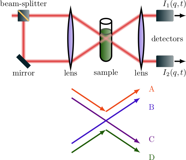
Figure 1.4: (a) Schematic representation of the side view (x-z-plane) of a 3D-DLS setup: A beam-slitter splits the laser beam into two beams that are vertically shifted. Both beams are scattered by the sample. Two photodetectors are in the same position in the x-y-plane but at different z-positions. (b) illustrates the potential paths that the laser light can take before being detected at one of the two detectors. Path A and B represent the top beam getting scattered into the top or bottom detector, respectively. Path C and D represent the bottom beam getting scattered into the top or bottom detector, respectively.

Instead of analyzing the auto-correlation function corresponding to the signal at a single detector, the cross correlation function of \(I_1(q, t)\) and \(I_2(q, t)\) is determined [6]:

\[\begin{equation} g_2^{c}(q, \tau) = \frac{\left<I_1(q, t)I_2(q, t+\tau)\right>}{\left<I_1(q)\right>\left<I_2(q)\right>} = 1 + \beta^2\beta_{OV}^2\beta_{MS}^2\beta_T^2[g_1(q, \tau)]^2 \tag{1.12} \end{equation}\]

The factor \(\beta\) and the function \(g_1(q,\tau)\) are analogous to the 2D case. However, three additional correction factors appear: \(\beta_{OV}\) is the overlap factor and corrects for the fact that the two laser beams do not probe the exactly same scattering volume. \(\beta_{T}\) is the technique-factor and is equal to 0.5 for the setup shown in Fig. 1.4 (a). \(\beta_{MS}\) is the multiple scattering factor and takes into account, that only a fraction of the signal is due to single scattering. It is inverse proportional to the \(MSF\) and is calculated from the time averages over the detected intensity from single scattering \(I_1^S(q, t)\) and \(I_2^S(q, t)\) and from the overall scattering \(I_1(q, t)\) and \(I_2(q, t)\):

\[\begin{equation} \beta_{MS} = \frac{\left<I_1^S(q)\right>\left<I_2^S(q)\right>}{\left<I_1(q)\right>\left<I_2(q)\right>} \tag{1.13} \end{equation}\]

Unlike the other \(\beta\)-factors, \(\beta_{MS}\) is \(q\)-dependent as it depends on \(I_{1/2}^S(q, t)\) and \(I_{1,2}(q, t)\) at the chosen \(q\)-value. Thus, it is indicative of the overall scattering strength: The more strongly the sample scatters, the higher the \(MSF\) and the lower \(\beta_{MS}\).

1.2.3 Modulated cross-correlation dynamic light scattering

It is not ideal that about half of the detected signal (all the signal from paths A and D in Fig. 1.4 (b)) is noise. To improve the technique, there is modulated 3D-DLS (mod3D-DLS). The setup (Fig. 1.5) is enriched by two intensity modulators. This ensures that only one laser path is active at each point in time and, therefore, that all the detected signal corresponds to the same \(q\)-value. However, the data corresponding to relaxation times slower that the modulation time \(\tau_{mod}\), which contains information about small length scales, is lost.

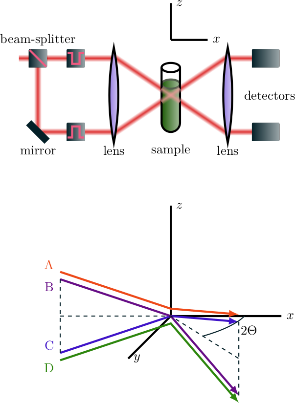
Figure 1.5: Schematic of the molulated 3D DLS setup. The two intensity modulators let only pass one laser beam at a time, while also only one detector detects.

The only differences in terms of data are higher quality (better signal-to-noise ratio) and a different \(\beta_T\) factor, namely \(\beta_T^2 = 0.85\).

1.2.4 Static Modulated Cross-correlation spectroscopy

The average scattered intensity will be a sum of single scattered photons and multiple scattering. \[\begin{equation} I(q) = I^s(q) + I^{MS}(q) \tag{1.14} \end{equation}\]

This measured intensity can be used together with \(\beta_{MS}\) from 3D-DLS to get the average scattering intensity of single scattered photons.

References

[1] W. Schärtl, Light Scattering from Polymer Solutions and Nanoparticle Dispersions, Springer Berlin Heidelberg, 2007.

[2] G. Galinsky, W. Burchard, Macromolecules 1997, 30, 6966.

[3] M. Medebach, C. Moitzi, N. Freiberger, O. Glatter, Journal of Colloid and Interface Science 2007, 305, 88.

[4] H. Lindner, G. Fritz, O. Glatter, Journal of Colloid and Interface Science 2001, 242, 239.

[5] I. D. Block, F. Scheffold, Review of Scientific Instruments 2010, 81, 123107.

[6] P. N. Pusey, Current Opinion in Colloid & Interface Science 1999, 4, 177.